---

There are two help screens for the Options tab for the one-way ANOVA dialog:

•A different page explains the multiple comparisons options.

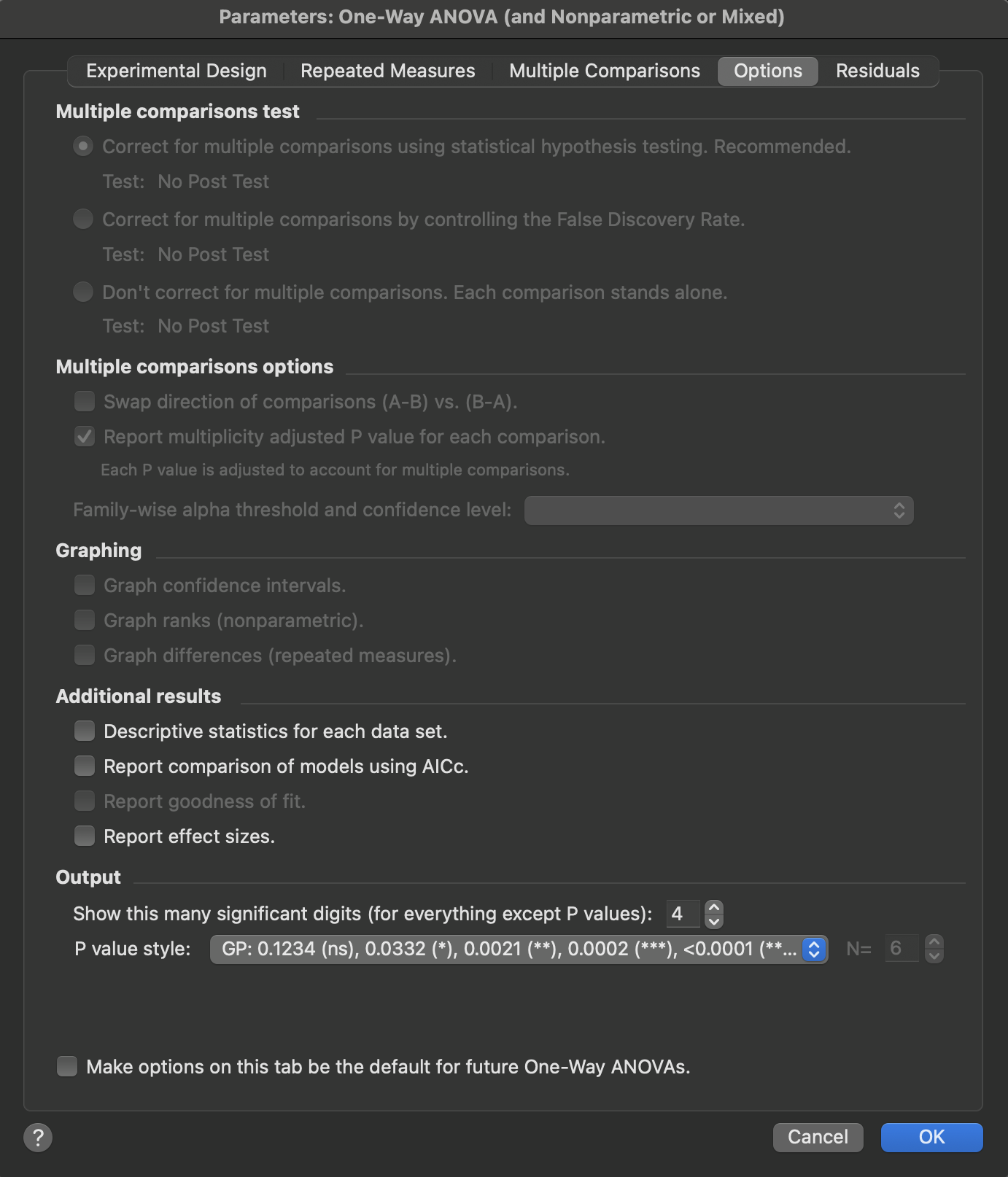
•This page explains the graphing and output options.

---

Graphing

Prism gives you options to create some extra graphs, each with its own extra page of results.

•If you chose a multiple comparison method that computes confidence intervals (Tukey, Dunnett, etc.) Prism can plot these confidence intervals.

•You can choose to plot the residuals. For ordinary ANOVA, each residual is the difference between a value and the mean value of that group. For repeated measures ANOVA, each residual is computed as the difference between a value and the mean of all values from that particular individual (row).

•If you chose the Kruskal-Wallis nonparametric test, Prism can plot the ranks of each value, since that is what the test actually analyzes.

•If you chose repeated measures ANOVA, Prism can plot the differences (for data sampled from a normal distribution) or log ratios (for data sampled from a lognormal distribution). If you have four treatments (A, B, C, D), there will be six set of differences (A-B, A-C, A-D, B-C, B-D, C-D) or ratios (A/B, A/C, A/D, B/C, B/D, C/D). Seeing these relationships graphed can give you a better feel for the data.

Additional results

•You can choose an extra page of results showing descriptive statistics for each column, similar to what the Column statistics analysis reports.

•Prism also can report the overall ANOVA comparison using the information theory approach (AICc), in addition to the usual P value. Prism fits two models to the data -- one where all the groups are sampled from populations with identical means, and one with separate means -- and tells you the likelihood that each is correct. This is not a standard way to view ANOVA results, but it can be informative.

Effect sizes

Prism can calculate effect sizes that quantify the magnitude of differences detected by one-way ANOVA. While P values tell you whether differences are statistically significant, effect sizes help you understand how large and meaningful those differences are. While some explanation is provided in the sections below, the page Understanding ANOVA Effect Sizes provides some additional details on the calculation and interpretation of standard effect sizes used in ANOVA. Prism reports several complementary effect size measures for one-way ANOVA:

% of total variation

This is the most intuitive effect size, expressing what percentage of the total variability in your data is explained by differences among group means. For example, if this value is 45%, it means that 45% of the variation in your data can be attributed to which group each value belongs to, while the remaining 55% is due to variability within groups.

Eta-squared (η²) and partial eta-squared

Eta-squared is mathematically equivalent to "% of total variation" but expressed as a proportion (0 to 1) rather than a percentage. For one-way ANOVA, eta-squared and partial eta-squared are identical since there is only one factor. These measures are widely used in psychological and social science research.

These values can be calculated from the ANOVA table with the following formulas:

Note that for one-way ANOVA, these two values are always equal as SS_effect + SS_error = SS_total. This is not true for higher order ANOVA models.

Cohen's f

Cohen's f is derived from eta-squared and provides standardized benchmarks for interpreting effect magnitude. Cohen suggested these guidelines:

•Small effect: f ≈ 0.10 (1% of variance explained)

•Medium effect: f ≈ 0.25 (6% of variance explained)

•Large effect: f ≈ 0.40 (14% of variance explained)

Cohen's f is particularly useful for power analysis and planning future studies, as it directly relates to the sample size needed to detect effects of a given magnitude.

Cohen's f can be calculated from eta squared or partial eta squared using the following formulas:

Since eta squared and partial eta squared are equal for one-way ANOVA, it doesn't matter which of these versions of the definition you use.

Interpreting effect sizes

When interpreting these effect sizes, consider both the statistical and practical significance of your results. A statistically significant P value with a small effect size might indicate a real but minor difference, while a large effect size (even if not statistically significant due to small sample size) might warrant further investigation. Effect sizes are particularly valuable when comparing results across studies or when conducting meta-analyses.

Output

Choose how you want P values reported, and how many significant digits you need.