1. Create a contingency table

From the Welcome or New table dialog, choose the contingency tab.

If you are not ready to enter your own data, choose one of the sample data sets.

2. Enter data

Most contingency tables have two rows (two groups) and two columns (two possible outcomes), but Prism lets you enter tables with any number of rows and columns.

You must enter data in the form of a contingency table. Prism cannot cross-tabulate raw data to create a contingency table.

For calculation of P values, the order of rows and columns does not matter. But it does matter for calculations of relative risk, odds ratio, etc. Use the sample data to see how the data should be organized.

Be sure to enter data as a contingency table. The categories defining the rows and columns must be mutually exclusive, with each subject (or experimental unit) contributing to one cell only. In each cell, enter the number of subjects actually observed. Your results will be completely meaningless if you enter averages, percentages or rates. You must enter the actual number of subjects, objects, events. For this reason, Prism won't let you enter a decimal point when entering values into a contingency table.

If your experimental design matched patients and controls, you should not analyze your data with contingency tables. Instead you should use McNemar's test.  

If you want to compare an observe distribution of values with a distribution expected by theory, do not use a contingency table. Prism offers another analysis for that purpose.

3. Analyze

From the data table, click on the toolbar, and choose Chi-square (and Fisher's exact) test.

Main calculations for tables with two rows and two columns

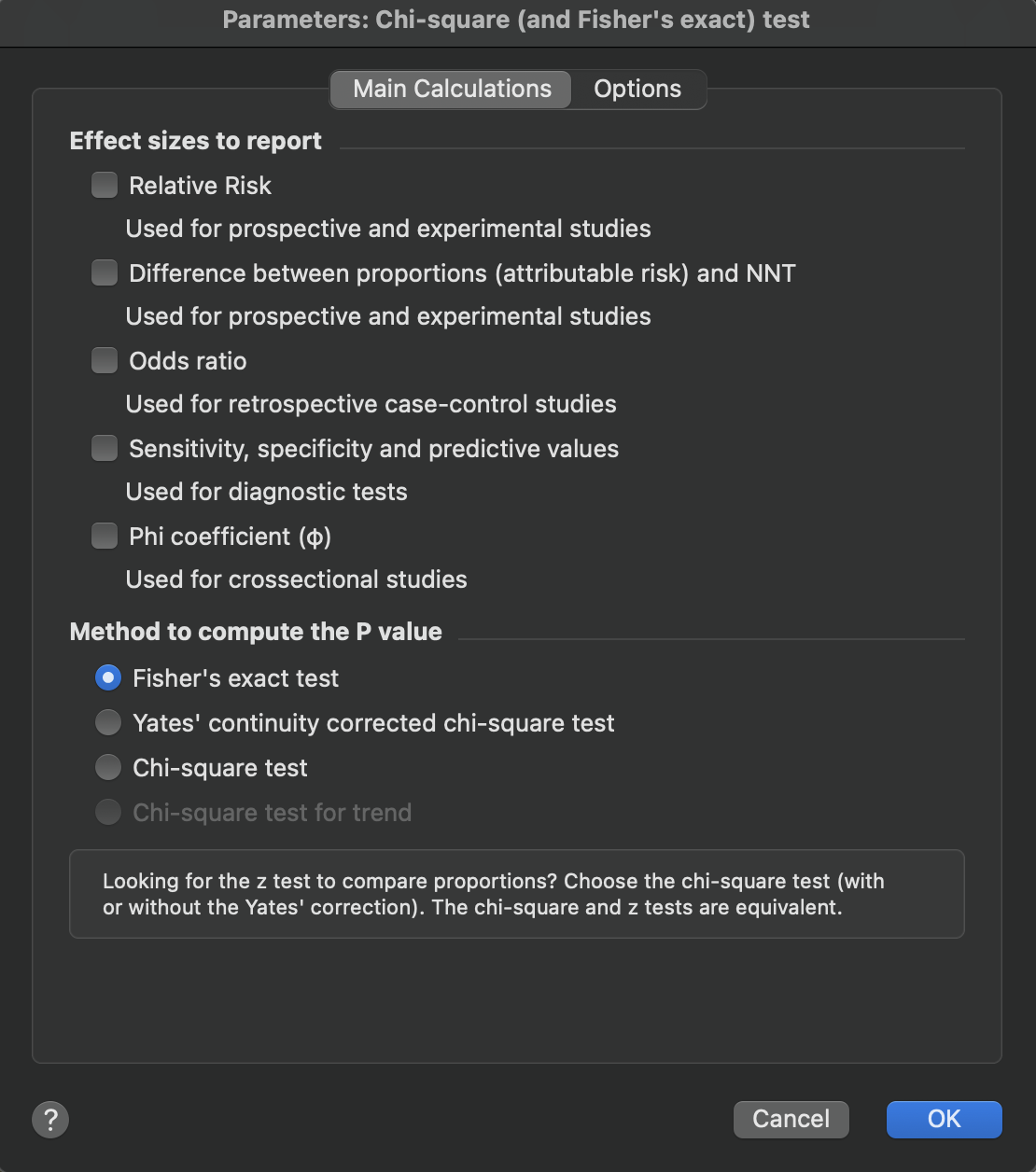
Your choice of effect sizes will depend on experimental design. Calculate an Odds ratio from retrospective case-control data, sensitivity (etc.) from a study of a diagnostic test, and relative risk and difference between proportions from prospective and experimental studies. All of these effect sizes apply only to 2x2 tables, so the choices will be gray if your table is larger.

If your table has two rows and two columns, we suggest you always choose Fisher's exact test to calculate the P value.

Main calculations for tables with more than two rows and/or more than two columns

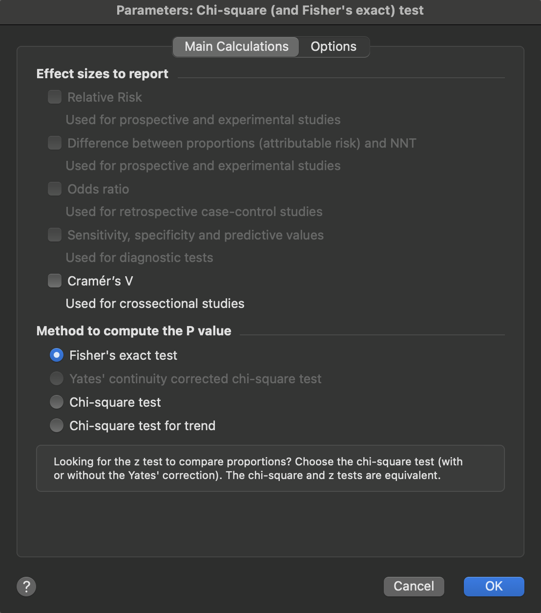
If your table has two columns and three or more rows, you can choose the chi-square test, Fisher's exact test, or the chi-square test for trend. This calculation tests whether there is a linear trend between row number and the fraction of subjects in the left column. It only makes sense when the rows are arranged in a natural order (such as by age, dose, or time), and are equally spaced. The test is also called the Cochran-Armitage test for trend. It is explained clearly, with equations and an example, on pages 261-265 Altman (2). You can find these pages at Google Books.

With contingency tables with more than two rows or columns, Prism always offers the choice to perform the chi-square test. Beginning with Prism version 10.1.0, Prism can also perform Fisher's exact test using extensions developed for this test to support larger tables.

Effect sizes for contingency tables

In addition to the effect sizes available for 2x2 tables (relative risk, odds ratio, etc.), Prism can calculate effect sizes that measure the strength of association in contingency tables of any size. These effect sizes help you understand not just whether an association exists (which the P value tells you), but how strong that association is.

Prism offers two related effect size measures:

•Phi coefficient (φ): Used for 2x2 contingency tables. The phi coefficient ranges from 0 (no association) to 1 (perfect association), and provides a standardized measure of effect size for crosssectional studies.

•Cramér's V: Used for larger contingency tables (more than 2 rows or columns). Cramér's V is essentially a generalization of the phi coefficient that works with tables of any size. Like phi, it ranges from 0 to 1.

Both measures are calculated from the chi-square statistic and provide similar interpretations. For 2x2 tables, the phi coefficient and Cramér's V are mathematically equivalent.

Effect size interpretation guidelines (Cohen, 1988):

•Small effect: φ or V ≈ 0.10

•Medium effect: φ or V ≈ 0.30

•Large effect: φ or V ≈ 0.50

These effect sizes are particularly useful for crosssectional studies where other measures like relative risk or odds ratio may not be appropriate. They complement the P value by providing information about the magnitude of the association between variables.

Options

     

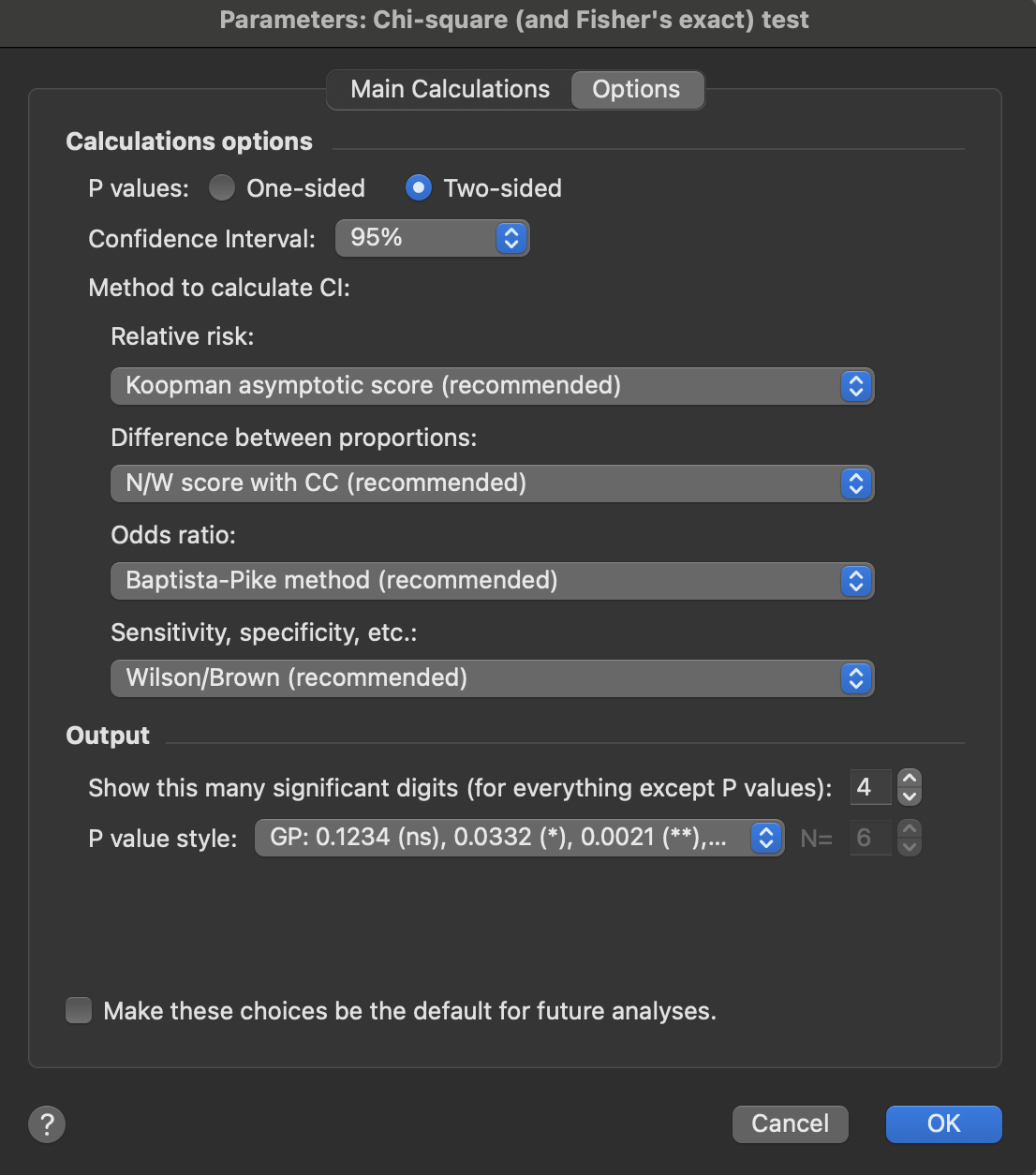
We suggest always choosing a two-sided P value unless you have a strong reason to choose a one-sided P value.  

Prism now offers a choice of method to use when computing confidence intervals.

•CI of the relative risk. The  method of Katz is an approximation, and we suggest not using it except to maintain compatibility with analyses done with earlier versions of Prism. There are many ways to compute the CI of a relative risk (1), and many of these seem good. Prism now offers the Koopman asymptotic score method, which we recommend.

•CI for the difference between proportions. The asymptotic method used by earlier versions of Prism is an approximation, and we suggest not using it except for compatibility. Instead choose the Newcombe/Wilson method(2). We offer that method with and without the continuity correction, and recommend the variation with that correction.  

•CI of the odds ratio. The  method of Woolf used by Prism 6 and earlier is an approixmation, and we suggest you not use it except to maintain compatibility. There are many good methods to compute the CI of an odds ratio (2). Prism now offers the Baptista-Pike method, which we recommend.

•CI of the sensitivity, specificity, etc. The so called "exact method" of Clopper and Pearson produces wide confidence intervals, and we suggest you don't use it except for compatibility. Instead choose the hybrid Wilson/Brown method (3).

You can also choose how you want P values formatted.

4. Review the results

Interpreting results: relative risk and odds ratio

Interpreting results: sensitivity and specificity

Interpreting results: P values (from contingency tables)

Analysis checklist: Contingency tables

 

1.Fagerland MW, Lydersen S, Laake P. Recommended confidence intervals for two independent binomial proportions. Stat Methods Med Res. SAGE Publications; 2011 Oct 13.

2.Newcombe, R. G. R. (1998). Interval estimation for the difference between independent proportions: comparison of eleven methods. Statistics in Medicine, 17(8), 873–890.  

3.Brown, L., Cai, T., & DasGupta, A. (2001). Interval Estimation for a Binomial Proportion. Statist. Sci, 16(2), 101–133.

4.Cohen, J. (1988). Statistical power analysis for the behavioral sciences (2nd ed.). Hillsdale, NJ: Lawrence Erlbaum Associates.