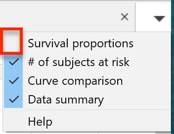
The analysis tab for survival proportions or percentages is invisible by default. It is used to make a graph, but you won't see the analysis tab until you turn it on in the analysis tab menu.

Survival proportions

Prism calculates survival proportions using the product limit (Kaplan-Meier) method. For each X value (time), Prism shows the fraction (or percentage) still alive (or the fraction or percentage already dead, if you chose to begin the curve at 0.0 rather than 1.0). This table contains the numbers used to graph survival vs. time.

The calculations take into account censored observations. Subjects whose data are censored--either because they left the study, or because the study ended -- can't contribute any information beyond the time of censoring. This makes the computation of survival percentage somewhat tricky. While it seems intuitive that the curve ought to end at a survival fraction computed as the total number of subjects who died divided by the total number of subjects, this is only correct if there are no censored data. If some subjects were censored, then subjects were not all followed for the same duration, so computation of the survival fraction is not straightforward (and what the Kaplan-Meier method is for).

If the time of death of some subjects is identical to the time of censoring for others, Prism does the computations assuming the deaths come first.

The results and graphs are labeled "Percent survival" but a more accurate term would be "Probability of survival". If there are any censored observations, the graph and table doesn't show percent survival in the experiment but rather probability of survival at any time given the censoring.

Confidence intervals of survival percentages

Prism reports the uncertainty of the fractional survival as a standard error or 95% confidence intervals. Standard errors are calculated by the method of Greenwood.

You can choose between two methods of computing the 95% confidence intervals:

•Asymmetrical method (recommended). It is computed using the log-log transform method, which has also been called the exponential Greenwood formula.  It is explained on page 42 and page 43 of Machin (reference below). You will get the same results from the survfit R function by setting error to Greenwood and conf.type to log-log. These intervals apply to each time point. The idea is that at each time point, there is a 95% chance that the interval includes the true population survival. We call the method asymmetrical because the distance that the interval extends above the survival time does not usually equal the distance it extends below. These are called pointwise confidence limits. It is also possible (but not by Prism) to compute confidence bands that have a 95% chance of containing the entire population survival curve. These confidence bands are wider than pointwise confidence limits.

•Symmetrical method. These intervals are computed as 1.96 times the standard error in each direction. In some cases the confidence interval calculated this way would start below 0.0 or end above 1.0 (or 100%). In these cases, the error bars are clipped to avoid impossible values. We provide this method only for compatibility with older versions of Prism, and don't recommend it.

How the Kaplan-Meier method works

The Kaplan-Meier method is logically simple. For each day (or week, however you scale the X values), it first computes the fraction of patients who are alive at the start of that day who survived until the end of that day. To do this, it simply divides the number alive at the end of that day by the number alive at the beginning of that day (excluding any who were censored on that day from both the numerator and the denominator).

Then it computes the fraction of patients who survived from day 0 until the end of each particular day. To do this, it multiplies the fraction of patients who survived Day 1 by the fraction of patients who were alive at the beginning of day 2 that survived until the end of Day 2 (excluding any censored), and then by the fraction of patients who were alive at the beginning of Day 3 that survived until the end Day 3 (excluding any censored), and so on, until you eventually multiply by the fraction who survived until the of Day k. The result of multiplying all these probabilities is the fraction of all patients who survived until the end of Day k, and this is the survival fraction that gets tabulated and graphed by Prism. This method automatically accounts for censored patients, because both the numerator and the denominator are reduced on the day a patient is censored. Because it calculates the product of many survival fractions, this method is also called the product-limit method.  

Reference

David Machin, Yin Bun Cheung, Mahesh Parmar, Survival Analysis: A Practical Approach, 2nd edition, IBSN:0470870400.