
Detecting outliers with Grubbs' test.
Statisticians have devised several ways to detect outliers. Grubbs' test is particularly easy to understand. This method is also called the ESD method (extreme studentized deviate).You can perform Grubbs' test using a free calculator on the GraphPad site. Prism 6 also has a built-in analysis that can detect outliers using Grubbs' method.
How Grubbs' test works
The first step is to quantify how far the outlier is from the others. Calculate the ratio Z as the difference between the outlier and the mean divided by the SD. If Z is large, the value is far from the others. Note that you calculate the mean and SD from all values, including the outlier.
Since 5% of the values in a Gaussian population are more than 1.96 standard deviations from the mean, your first thought might be to conclude that the outlier comes from a different population if Z is greater than 1.96. This approach only works if you know the population mean and SD from other data. Although this is rarely the case in experimental science, it is often the case in quality control. You know the overall mean and SD from historical data, and want to know whether the latest value matches the others. This is the basis for quality control charts.
When analyzing experimental data, you don't know the SD of the population. Instead, you calculate the SD from the data. The presence of an outlier increases the calculated SD. Since the presence of an outlier increases both the numerator (difference between the value and the mean) and denominator (SD of all values), Z can not get as large as many expect. For example, if N=3, Z cannot be larger than 1.155 for any set of values. More generally, with a sample of N observations, Z can never get larger than .
.
Grubbs and others have tabulated critical values for Z which are tabulated below. The critical value increases with sample size, as expected. You'll find the needed equation here, if you want to do your own analyses.
If your calculated value of Z is greater than the critical value in the table, then the P value is less than 0.05. This means that there is less than a 5% chance that you'd encounter an outlier so far from the others (in either direction) by chance alone, if all the data were really sampled from a single Gaussian distribution. Note that the method only works for testing the most extreme value in the sample (if in doubt, calculate Z for all values, but only calculate a P value for Grubbs' test from the largest value of Z.
Note that the 5% significance level applies to experiments, not to values. If you set alpha to 5% with the Grubbs test, then if the data are all Gaussian there is a 5% chance that any particular experiment will have an outlier. It does not mean that each value has a 5% chance of being defined as an outlier.
What to do with outliers
Think carefully about what to do with outliers. The possibilities are:
- The value is interesting. If each value is from a different animal or person, identifying an outlier might be important. You may have discovered a polymorphism in a gene, or a new clinical syndrome. Don't throw out the data as an outlier until first thinking about whether the finding is interesting.
- The value is a mistake. Maybe something got pipetted twice. Maybe there was a chunk or a bubble instead of a homogenous suspension. Maybe digits got transposed in data analysis.
- The distribution is not Gaussian. Grubbs' test depends on that assumption. A common situation is to have data that follow a lognormal distribution. Such a distribution has a heavy tail, and it is easy to mistake extreme values as outliers.
- The value may simply be the tail of a Gaussian distribution. If you define alpha to be 5%, then you'll mistakenly identify an outlier in 5% of samples you test.
People tend to jump to the second conclusion (that the value is an error so should be removed from the analysis) too soon. Think about the other possibilities.
Detecting more than one outlier
If you decide to remove the outlier, you then may be tempted to run Grubbs' test again to see if there is a second outlier in your data. This does not work well. The main problem is called masking. See an example. This occurs when there really are two outliers, but the presence of both increases the SD so much that neither one can be detected.
Critical values for Grubbs' test. with alpha=5%
|
N |
Critical Z |
|
N |
Critical Z |
|
3 |
1.15 |
|
27 |
2.86 |
|
4 |
1.48 |
|
28 |
2.88 |
|
5 |
1.71 |
|
29 |
2.89 |
|
6 |
1.89 |
|
30 |
2.91 |
|
7 |
2.02 |
|
31 |
2.92 |
|
8 |
2.13 |
|
32 |
2.94 |
|
9 |
2.21 |
|
33 |
2.95 |
|
10 |
2.29 |
|
34 |
2.97 |
|
11 |
2.34 |
|
35 |
2.98 |
|
12 |
2.41 |
|
36 |
2.99 |
|
13 |
2.46 |
|
37 |
3.00 |
|
14 |
2.51 |
|
38 |
3.01 |
|
15 |
2.55 |
|
39 |
3.03 |
|
16 |
2.59 |
|
40 |
3.04 |
|
17 |
2.62 |
|
50 |
3.13 |
|
18 |
2.65 |
|
60 |
3.20 |
|
19 |
2.68 |
|
70 |
3.26 |
|
20 |
2.71 |
|
80 |
3.31 |
|
21 |
2.73 |
|
90 |
3.35 |
|
22 |
2.76 |
|
100 |
3.38 |
|
23 |
2.78 |
|
110 |
3.42 |
|
24 |
2.80 |
|
120 |
3.44 |
|
25 |
2.82 |
|
130 |
3.47 |
|
26 |
2.84 |
|
140 |
3.49
|
Note that these values are for the two-sided Grubbs test. This looks for outliers that are either much higher than the other values or much lower. Prism and our QuickCalc only perform this two-sided Grubb's test. If your situation is such that an outlier can only be larger than the other values, and never smaller, then you can use a one-sided Grubb's test (which GraphPad doesn't offer). Grubb's paper (1) gives critical values for the one-sided test, but the values in the alpha=0.025 one sided test are also for the alpha=0.05 two sided test.
How the QuickCalcs calculator computes the critical value of the Grubs test
The QuickCalc outlier calculator uses the method documented in this page from the NIST. They use the variable G instead of the variable Z used above. The two have the same meaning. The key paragraph is:
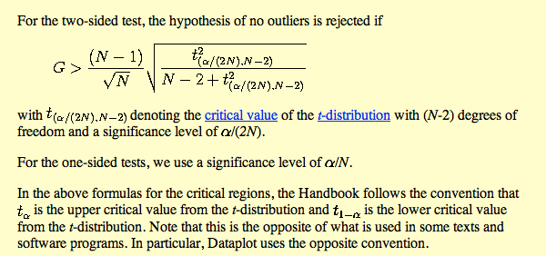
Computing an approximate P value
You can calculate an approximate P value as follows:
- Calculate

N is the number of values in the sample, Z is calculated for the suspected outlier as shown above.
- Look up the two-tailed P value for the student t distribution with the calculated value of T and N-2 degrees of freedom. Using Excel, the formula is =TDIST(T,DF,2) (the '2' is for a two-tailed P value). But note that this P value is not the P value of the Grubbs test. For that, continue to step 3.
- Multiply the P value you obtain in step 1 by N. The result is an approximate P value for the outlier test. This P value is the chance of observing one point so far from the others if the data were all sampled from a Gaussian distribution. If Z is large, this P value will be very accurate. With smaller values of Z, the calculated P value may be too large.
1. Grubbs, F. E. Procedures for detecting outlying observations in samples. Technometrics 11, 1–21 (1969).