The Gaussian distribution emerges when many independent random factors act in an additive manner to create variability. This is best seen by an example.
Imagine a very simple “experiment”. You pipette some water and weigh it. Your pipette is supposed to deliver 10 microliter of water, but in fact delivers randomly between 9.5 and 10.5 microliters. If you pipette one thousand times and create a frequency distribution histogram of the results, it will look like the figure below.
The average weight is 10 milligrams, the weight of 10 microliters of water (at least on earth). The distribution is flat, with no hint of a Gaussian distribution.
Now let's make the experiment more complicated. We pipette twice and weigh the result. On average, the weight will now be 20 milligrams. But you expect the errors to cancel out some of the time. The figure below is what you get.
Each pipetting step has a flat random error. Add them up, and the distribution is not flat. For example, you'll get weights near 21 mg only if both pipetting steps err substantially in the same direction, and that is rare.
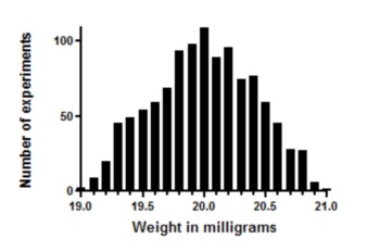
Now let's extend this to ten pipetting steps, and look at the distribution of the sums.

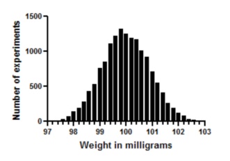
The distribution looks a lot like an ideal Gaussian distribution. Repeat the experiment 15,000 times rather than 1,000 and you get even closer to a Gaussian distribution.
This simulation demonstrates a principle that can also be mathematically proven. Scatter will approximate a Gaussian distribution if your experimental scatter has numerous sources that are additive and of nearly equal weight, and the sample size is large.
The Gaussian distribution is a mathematical ideal. Few biological distributions, if any, really follow the Gaussian distribution. The Gaussian distribution extends from negative infinity to positive infinity. If the weights in the example above really were to follow a Gaussian distribution, there would be some chance (albeit very small) that the weight is negative. Since weights can't be negative, the distribution cannot be exactly Gaussian. But it is close enough to Gaussian to make it OK to use statistical methods (like t tests and regression) that assume a Gaussian distribution.